Project description

Given task

In this exercise you will generate an inviscid, 2-D computational grid around a modified NACA 00xx series airfoil in a channel. The thickness distribution of a modified NACA 00xx series airfoil is given by:

\[y(x) = \pm 5t [0.2969 \sqrt{x_{int}x} - 0.126 x_{int} x - 0.3516 (x_{int}x)^{2} + 0.2843(x_{int}x)^{3} - 0.1015 (x_{int}x)^{4}]\]

where the “\(+\)” sign is used for the upper half of the airfoil, the “\(-\)” sign is used for the lower half and \(x_{int} = 1.008930411365\). Note that in the expression above \(x\), \(y\), and \(t\) represent values which have been normalized by the airfoil by the airf oil chord.

A sketch of the computational domain is shown below:

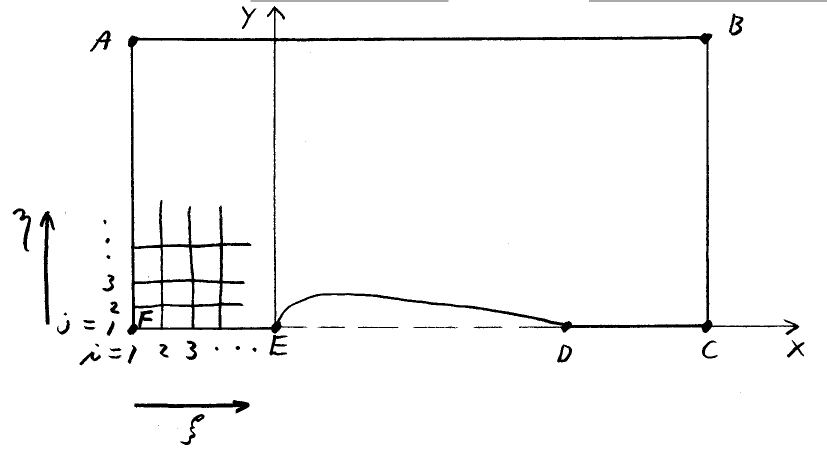
Each grid point can be described by \((x,y)\) location or \((i,j)\) location where \(i\) is the index in the \(\xi\) direction and the \(j\) index is in the \(\eta\) direction. The grid should have imax=41 points in the \(\xi\) direction and jmax=19 points in the \(\eta\) direction. The coordinates of points A-F shown in the figure are given in the following table:

Point	\((i,j)\)	\((x,y)\)
A	(1,19)	(-0.8,1.0)
B	(41,19)	(1.8,1.0)
C	(41,1)	(1.8,0.0)
D	(31,1)	(1.0,0.0)	(trailing edge)
E	(11,1)	(0.0,0.0)	(leading edge)
F	(1,1)	(-0.8,0.0)

Algebraic Grid

To complete this project you will first generate a grid using algebraic methods. Use uniform spacing in the \(x\) direction along FE, along ED, and along DC. (However, note that the spacing in the \(x\) direction along FE and DC will be different from the spacing along ED). Use uniform spacing in the \(x\) direction along AB. (However, note that the spacing in the \(x\) direction along AB will be different from that along FE, ED, and DC). For the interior points of the initial algebraic grid use a linear interpolation (in computational space) of the boundary \(x\) values:

\[x(i,j) = x(i,1) + \left ( \frac{j-1}{jmax-1} \right ) [x(i,jmax) - x(i,1)]\]

Use the following stretching formula to define the spacing in the \(y\) direction:

\[y(i,j) = y(i,1) - \frac{y(i,jmax)-y(i,1)}{C_{y}} ln \left [ 1 + (e^{-C_{y}} - 1) \left ( \frac{j-1}{jmax-1} \right ) \right ]\]

where \(C_{y}\) is a parameter that controls the amount of grid clustering in the \(y\)-direction. (If nearly uniform spacing were desired we would use \(C_{y}\) = 0.001).

The algebraic grid generated now serves as the initial condition for the subroutines which generate the elliptic grid. The bounday values of the initial algebraic grid will be the same as those of the final elliptic grid.

Elliptic Grid

The elliptic grid will be generated by solving Poisson Equations:

\[\xi_{xx} + \xi_{yy} = P(\xi,\eta)\]\[\eta_{xx} + \eta_{yy} = Q(\xi,\eta)\]

where the source terms,

\[A_{1} (x_{\xi\xi} + \phi x_{\xi}) - 2A_{2} x_{\xi\eta} + A_{3}(x_{\eta\eta} + \psi x_{\eta}) = 0\]\[A_{1} (y_{\xi\xi} + \phi y_{\xi}) - 2A_{2} y_{\xi\eta} + A_{3}(y_{\eta\eta} + \psi y_{\eta}) = 0\]

where the \(A\)‘s must be defined by mathmatical manipulation.

On the boundaries, \(\phi\) and \(\psi\) are defined as follows:

\[\begin{split}\text{On } j = 1 \text{ and } j = jmax: \text{ }\phi = \begin{cases} -\frac{x_{\xi\xi}}{x_{\xi}} & \text{ if } |x_{\xi}| > |y_{\xi}| \\ -\frac{y_{\xi\xi}}{y_{\xi}} & \text{ if } |x_{\xi}| \leq |y_{\xi}| \end{cases}\end{split}\]\[\begin{split}\text{On } i = 1 \text{ and } i = imax: \text{ }\psi = \begin{cases} -\frac{x_{\eta\eta}}{x_{\eta}} & \text{ if } |x_{\eta}| > |y_{\eta}| \\ -\frac{y_{\eta\eta}}{y_{\eta}} & \text{ if } |x_{\eta}| \leq |y_{\eta}| \end{cases}\end{split}\]

At interior points, \(\phi\) and \(\psi\) are found by linear interpolation (in computational space) of these boundary values. For example,

\[\psi_{i,j} = \psi_{1,j} + \frac{i-1}{imax-1} \left ( \psi_{imax,j} - \psi_{1,j} \right )\]

Challenges

Demonstrate your solver by generating 5 grids (each with 41x19 grid points):

Grid #1

Initial algebraic grid, non-clustered (\(C_{y}\) = 0.001)

Grid #2

Initial algebraic grid, clustered (\(C_{y}\) = 2.0)

Grid #3

Elliptic grid, clustered (\(C_{y}\) = 2.0), no control terms (\(\phi\) = \(\psi\) = 0)

Grid #4

Elliptic grid, clustered (\(C_{y}\) = 2.0), with control terms

Grid #5

Now, use your program to generate the best grid you can for inviscid , subsonic flow in the geometry shown. You must keep imax = 41, jmax = 19 and not change the size or shape of the outer and wall boundaries. You may, however, change the grid spacing along any and all of the boundaries and use different levels of grid clustering wherever you think it is appropriate.