Code development
The current project is for developing elliptic grid generator in 3-dimensional domain. Hereafter, the program developed in this project is called ‘GridGen’.
GridGen Code summary
The present project is to make a grid-generator for 3-D computational domain around a modified NACA 00xx series airfoil in a channel. The assigned project is inherently aimed at 2-D grid. However, the currently built GridGen code has a capability of 3-D grid generation.
The source code contains two directories, ‘io’, and ‘main’, for input/output related sources and grid-setup related sources, respectively. ‘CMakeLists.txt’ file is also included for cmake compiling.
$ cd GridGen/CODEdev/src/
$ ls
$ CMakeLists.txt  io  main
The io folder has io.F90 file which contains ReadGridInput() and WriteTecPlot() subroutines. It also includes input directory which contains default input.dat file.
The main folder is only used for containing grid-setup related source files. The main routine is run by main.F90 which calls important subroutines from main folder itself and io folder when needed. All the fortran source files main folder contains are listed below:
> GridSetup.F90
> GridTransform.F90
> GridTransformSetup.F90
> main.F90
> Parameters.F90
> SimulationSetup.F90
> SimulationVars.F90
Details of GridGen development
The GridGen code is made for creating 3-D computational domain with pre-described points value along the 2D airfoil geometry. The schematic below shows the flow chart of how the GridGen code runs.
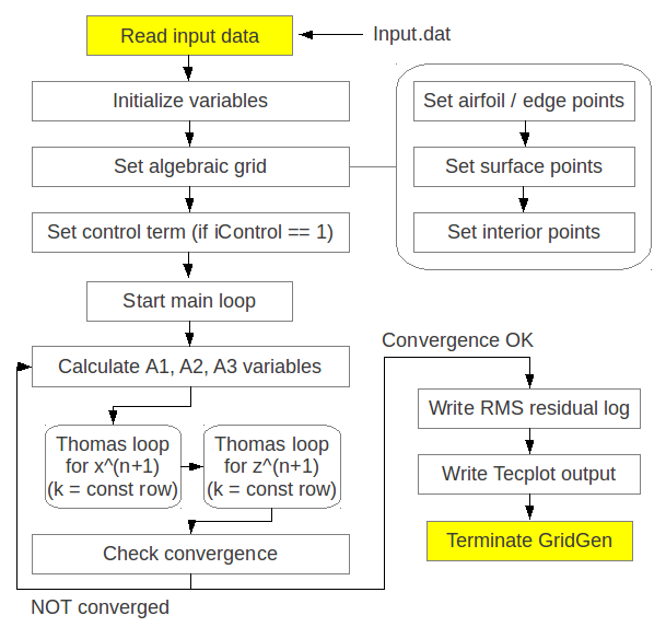
The source code shown below is main.F90 and it calls skeletal subroutines for generating grid structure. The main features of the main code is to (1) read input file, (2) make initialized variable arrays, (3) set initial algebraic grid points, (4) create elliptic grid points, and (5) finally write output files:
PROGRAM main
   USE SimulationSetup_m, ONLY: InitializeCommunication
   USE GridSetup_m, ONLY: InitializeGrid
   USE GridTransform_m, ONLY: GridTransform
   USE io_m, ONLY: WriteTecPlot, filenameLength
   USE Parameters_m, ONLY: wp

   IMPLICIT NONE

   CHARACTER(LEN=filenameLength) :: outputfile = 'output.tec'

   CALL InitializeCommunication
   ! Make initial condition for grid point alignment
   ! Using Algebraic method
   CALL InitializeGrid
   ! Use Elliptic grid points
   CALL GridTransform
   CALL WriteTecPlot(outputfile,'"I","J","K","Jacobian"')
END PROGRAM main
Creation of algebraic grid points
The code starts to run by reading the important input parameters defined in input.dat file. The input data file first contains the number of i, j, k directional grid points. Then the code reads airfoil geometry data from this input file, which provides the bottom edge points of the domain. The input file also contains four vertex points in \((x,y,z)\) coordinates. Thus those points forms a 2-dimensional surface, which is supposed to be created in this project. Next, the code clones these grid points and locates them away from this surface in \(j\)-direction, resulting in 3-dimensional computational domain. Based on these boundary grid points, the code runs with Algebratic grid generating subroutine and gives initial conditions for elliptic solution for grid transformation.
The main.F90 file first refers to InitializeGrid subroutine defined in GridSetup.F90 file. The main function of this routine is to call again multiple subroutines defined in same file. The subroutine definition shown below summarizes the how the code runs for the grid initialization:
!-----------------------------------------------------------------------------!
   SUBROUTINE InitializeGrid()
!-----------------------------------------------------------------------------!
   USE io_m, ONLY: ReadGridInput
   USE SimulationVars_m, ONLY: imax, jmax, kmax,&
                             xblkV, cy
   IMPLICIT NONE

   ! Create Bottom Edge coordinate values
   CALL ReadGridInput
   CALL InitializeGridArrays
   CALL CreateBottomEdge
   CALL SetEdgePnts
   CALL GridPntsAlgbra
   CALL GenerateInteriorPoints

   END SUBROUTINE
- ReadGridInput: Reads important user defined variables and parameters for grid configuration.
- InitializeGridArrays: Initialize the single- and multi-dimensional arrays and set their size with input parameters(for example, imax, jmax, kmax).
- CreateBottomEdge: Generate point values for airfoil geometry.
- SetEdgePnts: Generate grid points along 8 edges of the computational domain.
- GridPntsAlgbra: Based on the edge points, this routine will distribute grid points located on each 6 surfaces of the computational domain.
- GenerateInteriorPoints: Based on grid points along the edges and surfaces, this routine will create interior grid points that are aligned with user-defined grid point interpolations.
Creaction of elliptic grid points
In order to determine the elliptic grid points with the pre-specified boundary points, the following Poisson equations, which is given in previous Project description section, have to be resolved numerically. The coefficients of the equations can be determined by:
Then, applying finite difference approximation to the governing equations can be transformed into the linear system of equations. The arranged matrix form of equations shown below can be solved for unknown implicitly at every pseudo-time level. At every time loop, the code updates the coefficients composed of \(\phi\) and \(\psi\), and adjacent points. The detailed relations of each coefficients are not shown here for brevity.
Above equations can be numerically evaluated by the following descritized expressions:
where \(n\) and \(n+1\) indicate pseudo time index. Thus above equations will update grid point coordinates for \(n+1\) time level by referring to already resolved \(n\) time level solution. Note that the pseudo time looping goes along the successive \(j\)-constant lines. Therefore, when writing the code, time level index in above equations was not considered as a separate program variable because \(j-1\) constant line is already updated in the previous loop.
The expressions above are only evaluted in the interior grid points. The points on the boundaries are evaluated seprately by applying given solutions as problem handout.
Once initial algebraic grid points are created, the code is ready to make elliptic grid points with some control terms in terms of \(\phi\) and \(\psi\). GridTransform.F90 file contains a subroutine named by GridTransform as shown below:
!-----------------------------------------------------------------------------!
   SUBROUTINE GridTransform()
!-----------------------------------------------------------------------------!
   IMPLICIT NONE
   INTEGER :: n

   CALL InitializeArrays
   IF ( iControl == 1) CALL CalculatePiPsi
   DO n = 1, nmax
      CALL CalculateA123
      CALL ThomasLoop
      CALL WriteRMSlog(n,RMSlogfile)
      IF (RMSres <= RMScrit) EXIT
   ENDDO
   CALL CopyFrontTOBack
   CALL GenerateInteriorPoints
   CALL CalculateGridJacobian
   END SUBROUTINE GridTransform
Before going into the main loop for solving poisson equations, the code calculate control terms with \(\phi\) and \(\psi\). Even though the assigned project made an assumption of linear interpolated distribution of \(\phi\) and \(\psi\) at interior points, the GridGen code is designed to allow \(\phi\) and \(\psi\) be weighted in \(j\) and \(i\) directions, respectively. This effect is made by the grid stretching formula. This will be revisited for discussion on Grid 5.
Here, main DO-loop routine goes with setup of coefficients of governing equations and Thomas loop. The Thomas loop operates with line Gauss-Siedel method for resolving unknown variables, \(x\) and \(y\), with tri-diagonal matrix of coefficients of finite difference approximation equation in a \(k\) = constant line. Note that the GridGen code transforms the grid points with elliptic solution only in front surface, then clones the grid points to the back surface and finally creates interior points. The front surface is made up of \(i\) and \(k\) coordinates.
Write Convergence history: RMS residual
In order to avoid infinite time-looping for the Thomas method, the GridGen code employs the following definition of RMS residual based on the new (\(n+1\)) and old(\(n\)) values of grid point coordinates.
where \(N = 2x(\text{imax}-2) x (\text{jmax}-2)\) and the RMS criterion is pre-specified as: \(1\text{x}10^{-6}\). In this code, the convergend is assumed to be achived when RMS residual is less than the RMS criterion.